Meeting No. 3

Data Analysis:

The simulation for the 330MeV is not done yet. It takes more time than expected. The next iteration will probably be finished today/tomorrow. Next I will start analysis for 495MeV, which will take another week of time.

What do you think/see?

The two plots show my latest results for the 330MeV. I checked my code and I do not have much room for the improvement, ie. extra removal of the background. The Snout contributions seem ok, so do the TG corrections.

If I look at the first plot, which is normalized to the elastic run, I see a systematic rise (except of the last data point), which indicates, that backgrounds are not considered properly.

0A.)

If I renormalize the 330MeV data to the average of the ratio (excluding elastic point), I see the oscillation (what already Harald observed already last week), which is somehow consistent with the oscillation of the 195MeV data.

0B.)

Simulation for Lupolen target

This analysis was put on hold this week. I have only talked to Florian, who is willing to install Lupolen target for a potential short test in February. Will this be possible?

Optics for Spectrometer A with 12C data:

I was working on the optics for spectrometer A. I have started with the 360MeV Carbon data, because the data sample is smaller. I did not find any serious mistake in my previous analysis and I am still not sure why the analysis did not work before. Now it seems to be working reasonably well. At the moment I am working with the "Fast" algorithm, which throws all the unnecessary elements away in a single iteration.

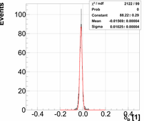
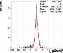
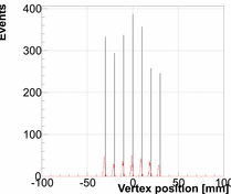
I have tested the matrix first on the points used for calibration (directly from the gridfinder). The results I get are ok. The angular resolutions are consistent with the values from the NIM paper, the values for delta and y0 are approx. 1-2x worse. Resolution is more 2E-4 and not 1E-4, but results my improve when more matrix elements will be considered.

01.)

02.)

03.)

04.)

05.)

06.)

07.)

08.)

09.)

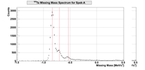
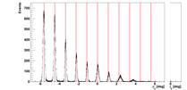
Then I tested matrix on the full data. The resolutions worsen a bit more, which was expected, but not much:

10.)

11.)

12.)

13.)

14.)

15.)

16.)

17.)

18.)

19.)

20.)

21.)

22.)

23.)

From the results above, one can see, that everything works well, except of the variable phi0 at phi0>0. Phi0>0 means large scattering angles. These data have limited statistics, because the data were taken at the end of the experiment. At large scattering angles, the CS is small and statistics is low. I made my gridfinder analysis with threshold 0.1, which throws all the data points at phi0>0 away. Since no calibration data points, the reconstruction does not work there. To remove this problem, I repeated the analysis with threshold at 0.01, and now I have more data points. However, the algorithm is still working and the results will be ready next week.

Determination of Offsets:

Before being able to calculate the matrix, the offsets from the Fp variables need to be removed. The plots below show the results and the comparison with the results from the Ta analysis at 495MeV.

24.)

25.)

26.)

Optics for Spectrometer A with 181Ta data:

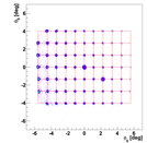
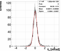
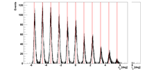
We have much better data with 181Ta target. So far I have been able to determine the gridfinder tables. Now I need to run my SVD algorithm to determine the matrices. Since we have much larger data sample here, the analysis is much slower. I have been able to do first tests, and while the resolution in delta is still inferior, the results for phi0 and y0 are much better:

27.)

28.)

29.)

30.)

31.)

32.)

33.)

34.)

35.)

36.)

37.)

38.)

39.)

40.)

41.)

I first need to check the results of the optics with large matrices and FastSVD algorithm. Once I am happy with the results I will repeat the procedure with the Full (precise) SVD algorithm and determined the final matrices. I still need to check, where this 1E-16 limit in the p-values comes from. Then I will repeat the procedure for the spectrometer B. At the end I will also analyze the data at the 195MeV, taken in 2014. Hence, at the end we will have matrices for all three beam energies - and hopefully a NIM-A paper.