Meeting No. 21
Correspondence with Doug Higinbotham
Before Christmas I exchanged few emails with Douglas Higinbotham, who
fitted our results in his own way and got the same results as we do (in his units).
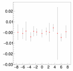
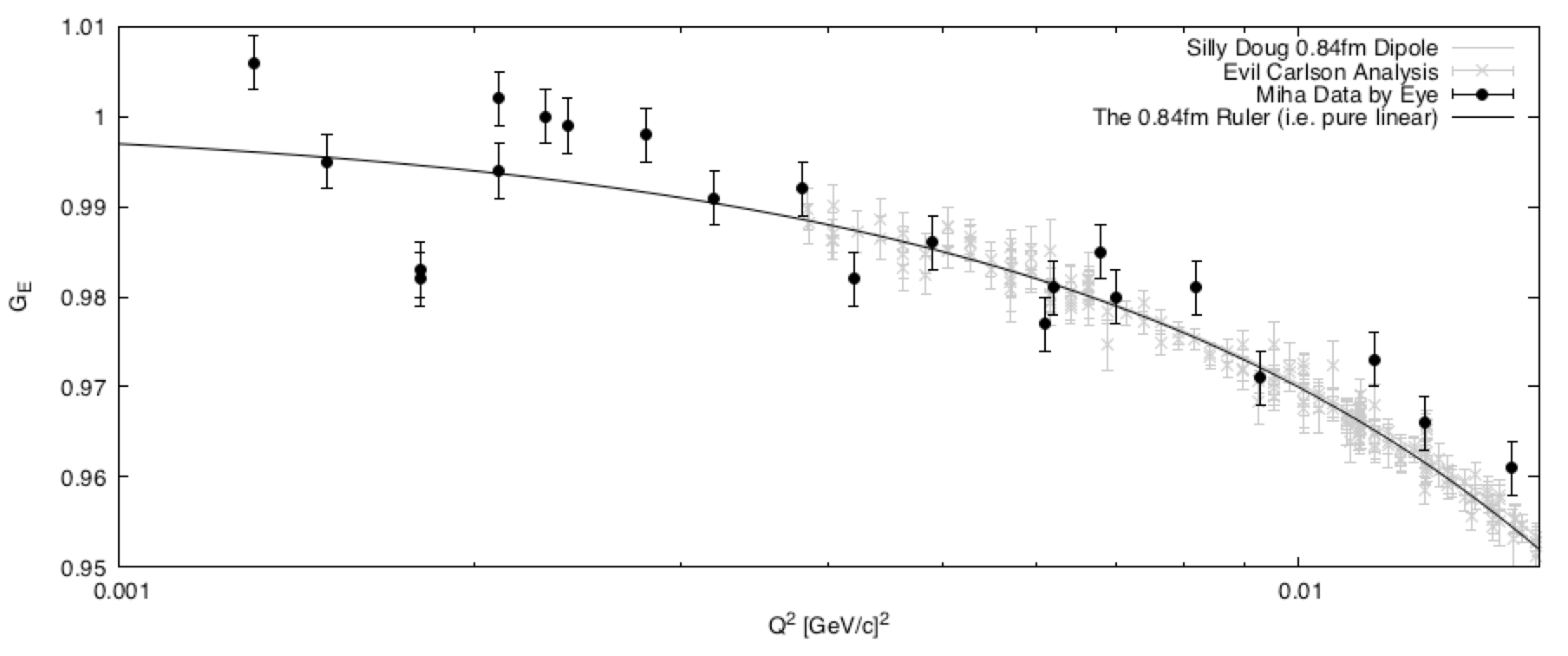
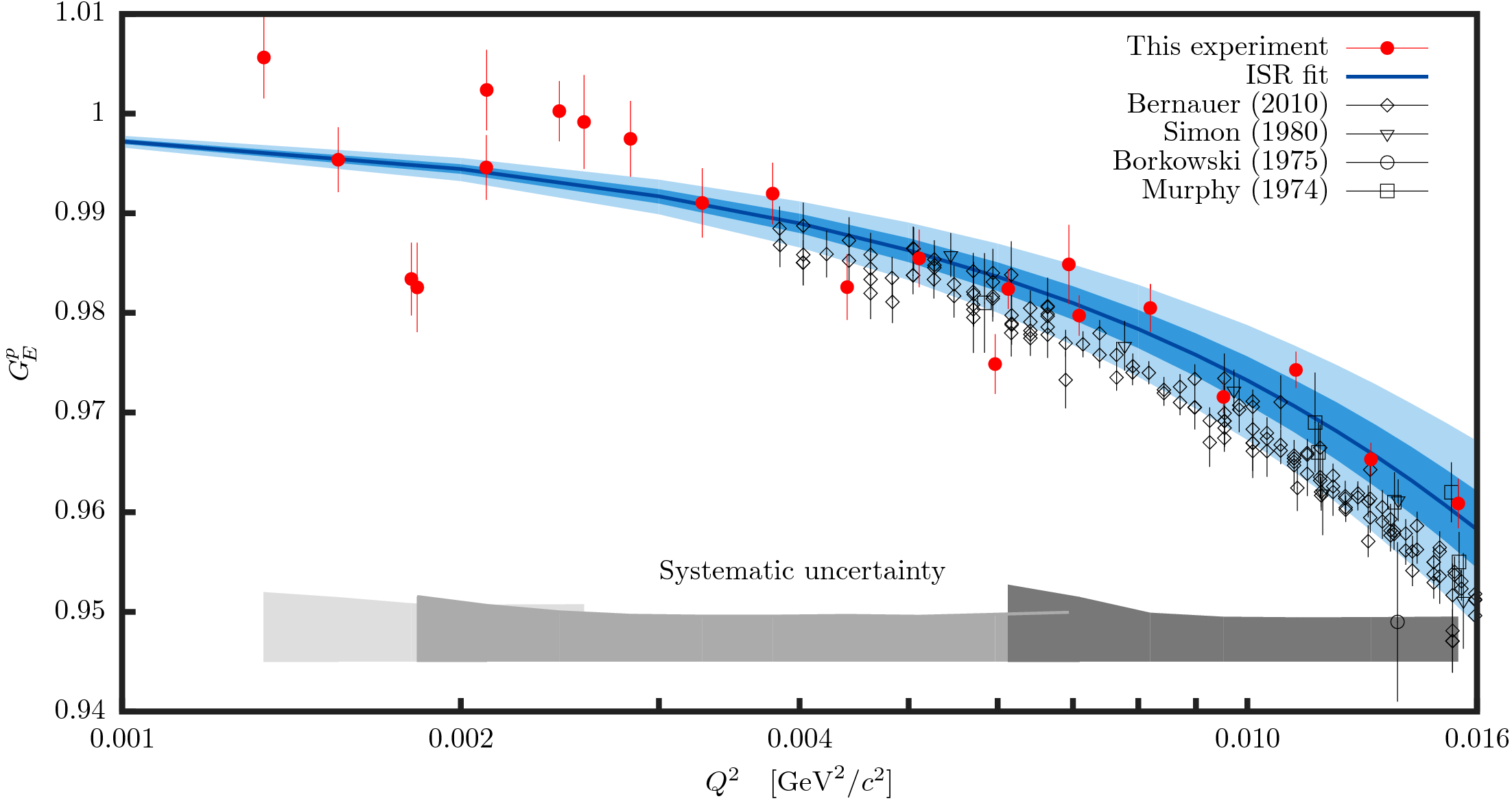
His radius goes from 0.7fm to 0.9fm. He also suggested to change our plot, to make
our contribution to the community more pronounced. He would change the linear scale
to logarithmic to stretch our points (although he was the first in favor of the linear scale).
Furthermore, it shows more clearly that there is curvature in the fit.
01.)  02.)
02.) 
03.) 
I find this suggestion useful and therefore followed the suggestion and made a new plot.
Here are the old and the new version.
04.)  05.)
05.) 
He was a bit disappointed that in the paper we did not mention other "fitters" and pRad experiment.
I tried to explain, that we do not have space to do that!
Lupolen data and problem with External Radiation Corrections
Since we are going to investigate the external radiation corrections with a
Lupolen target, I revisited my analysis from February and tried to learn more from
that data. For that purpose I improved the simulation. I included the generator for
the Lupolen and added excited states for Carbon and Tantal.
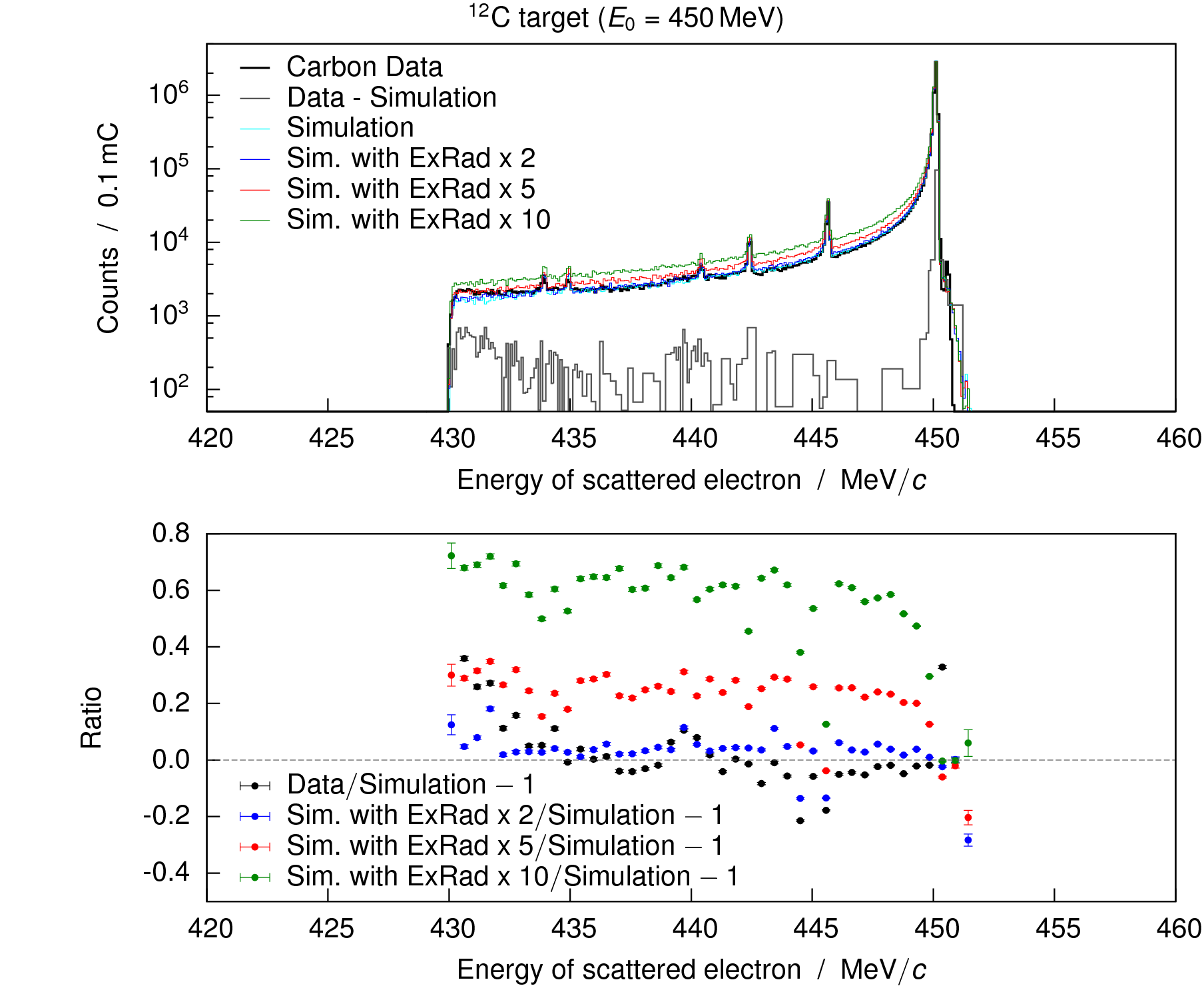
Then I first inspected Carbon data. Here I encountered a problem, that the peaks were much
broader than expected. This was due to the large wobbler in the vertical direction
that distorts the optics in B. Since linear dependence, I could correct for that. However,
in the next experiment, we should not wobble in vertical direction!!! It is a problem.
I got results shown in the plot below. Then I changed the contribution of the external
radiative corrections to see the size of the effect. It is small, since the target is
thin! Furthermore, it is hard to separate resolution effects and the external radiative corrections.
06.) 
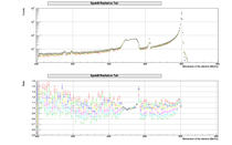
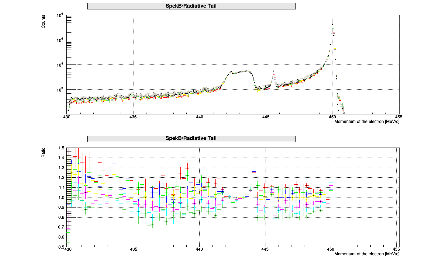
Then I investigated Lupolen target. Here the resolution does not play such a strong role, since
Hydrogen has broader recoil correction. Here one can see, that with the given implementation of
radiative corrections something is missing in the first part of the Hydrogen tail. Similarly
to what we see in the ISR experiment.
07.) 
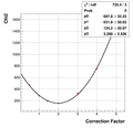
This can be compensated for, if we increase the external corrections. Plots below show, for which factor
we need to increase the relative thickness of the material, in order to get the best match. It is approx. 2.
I also investigated how the result changes if I lower the resolution from 0.000085 to 0.00017. Not significantly.
Still something is missing.
08.)  09.)
09.) 
10.)  11.)
11.) 
Now I am working on the 195MeV data with spectrometer A. Here more excited states (and other stuff) is present.
Hence, simulation does not work that well. In the one also sees the problems with the optics, since the peaks are not
properly aligned. Hence, I am trying a different method in order to see, if I see here the same effect. Work in progress!
12.) 
New Target
What kind of target shell we design for the February beam time? Simply a thick Lupolen to enhance
the effect of external radiative corrections, or ladder with different thicknesses! I am in favor of the
last option. Do we have Lupolen available?
Calibration of Spec-B at @ 360MeV
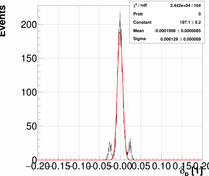
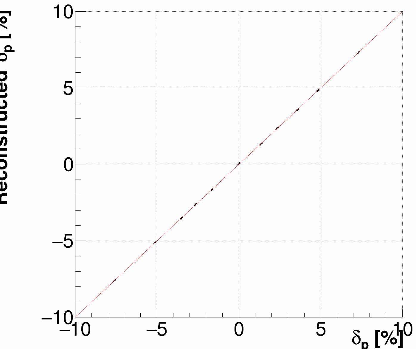
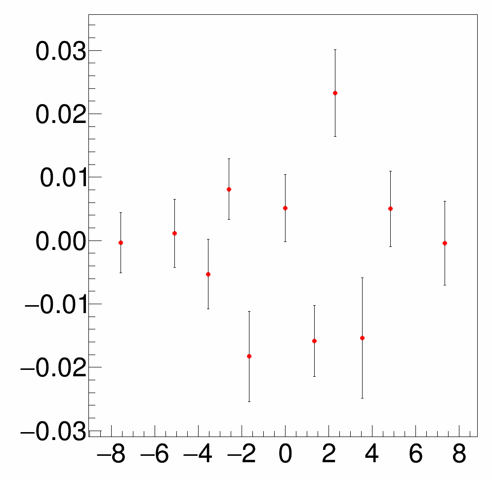
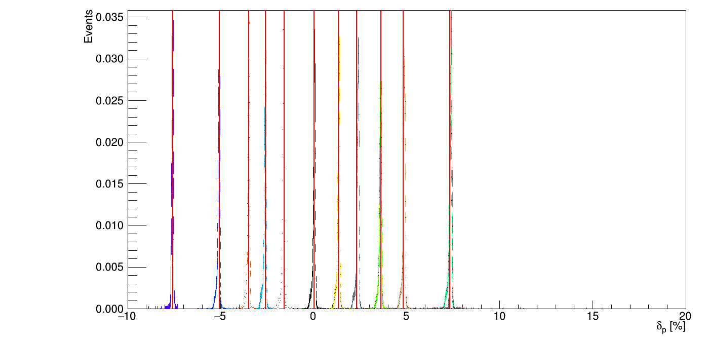
The optics calibration of the 495MeV and 195MeV data is done. However, I am still struggling with the
360MeV settings. From the plots below one can see, that results are not as good as for the 495MeV setting.
Almost for factor 5 better!!!
Analysis of the 360MeV data (full set)
13.)  14.)
14.) 
15.)  16.)
16.) 
17.) 
For comparison results for 495MeV setting
18.)  19.)
19.) 
20.)  21.)
21.) 
Problem with the NMR
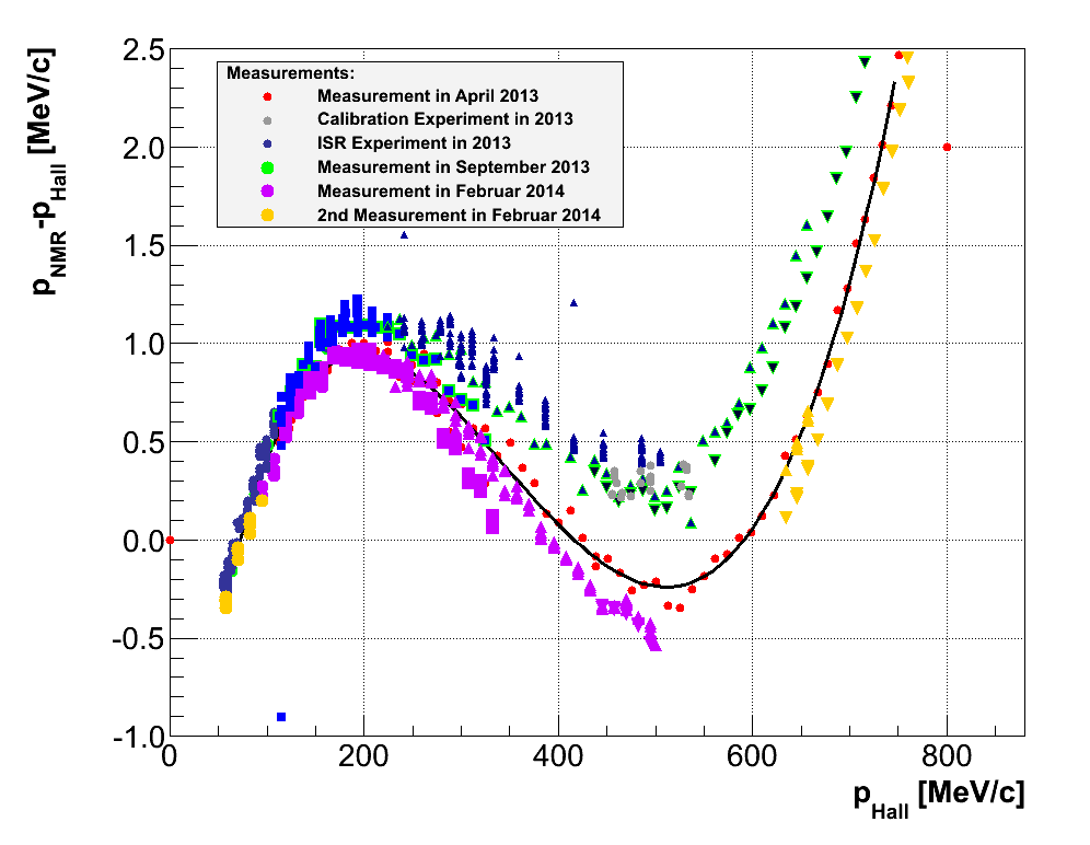
I believe, this has to do with the fact, how well can we position spectrometer B. In the bottom plot one can
see, that while at 200MeV and 500MeV the NMR readouts are stable and offset between NMR and Hall probe are
constant, at 360MeV we are at the maximum of the slope. This causes the problems and the fluctuations of the
results.
22.) 
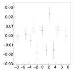
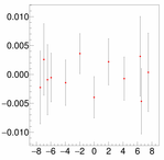
Interestingly the difference between the NMR and Hall probe has the same trend as the difference
between the reconstructed and exact value of the delta! Red points are (NMR-HALL)/HALL. The blue points
are differences between the determined delta and delta obtained with good matrix (495MeV taken as
absolute truth), Green points are obtained with 360MeV matrix. Ideally, this points should all lie at 1.
23.) 
Analysis of the 360MeV data (including 4.4MeV and 9.6 MeV excited states)
I tried to make my matrix more robust by including excited states at 4.4MeV and 9.6 MeV. The results improve although still not good!
24.)  25.)
25.) 
26.)  27.)
27.) 
28.) 
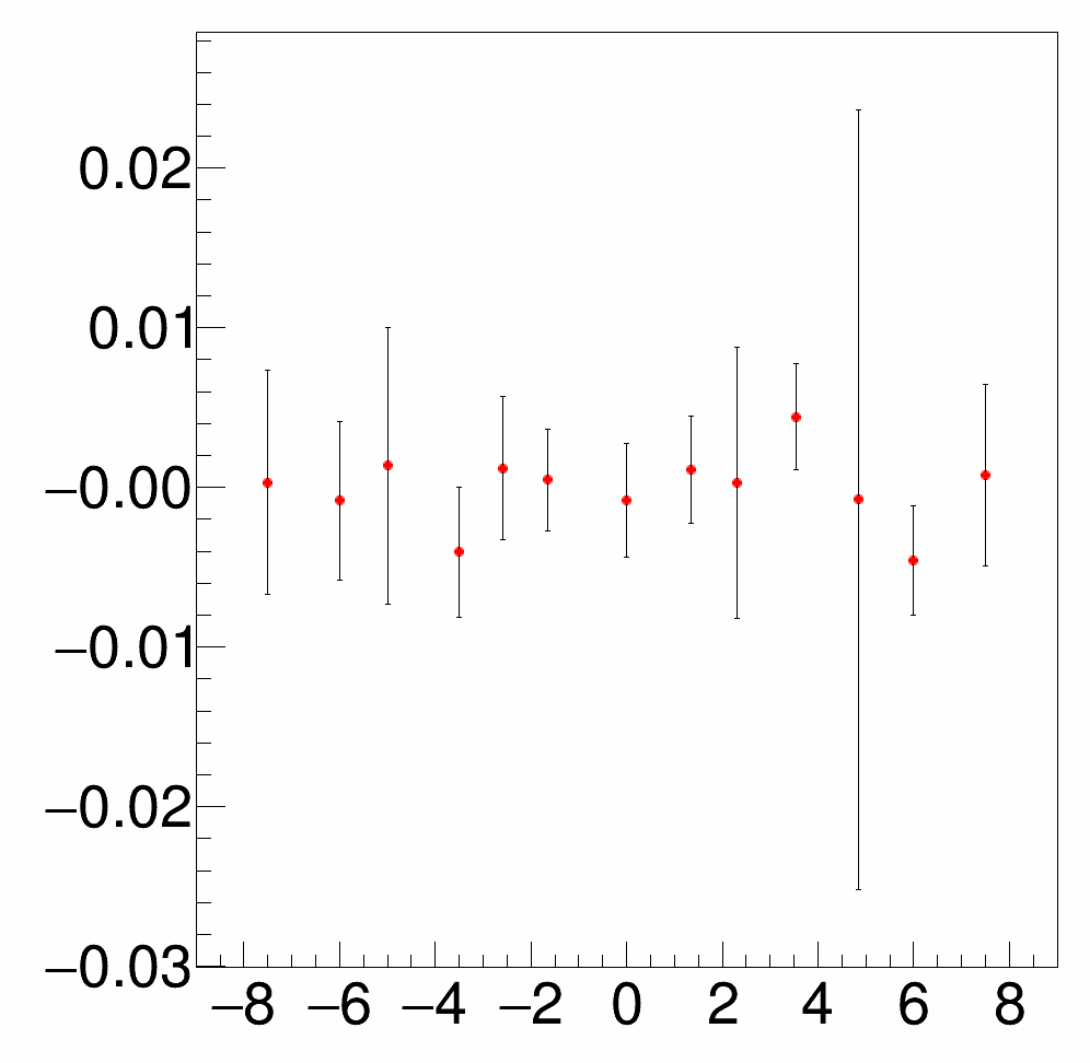
Indeed problem of moving magnet up and down
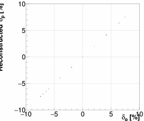
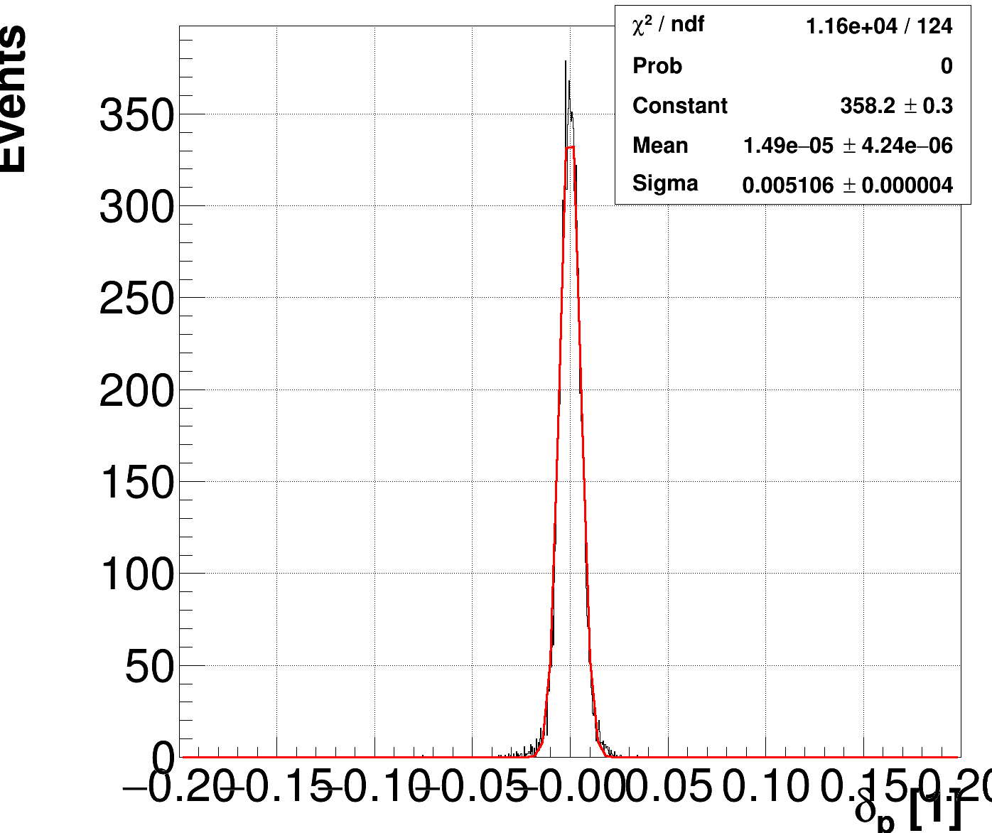
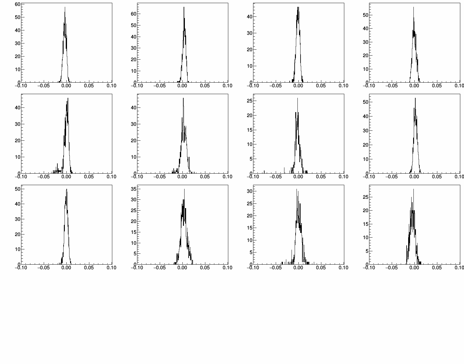
Looking at the reconstructed peaks one can see that they fall into three groups. Isolating one group I
believe I identified the problem, which is really correlated with the fact, how well we can determine the central momentum, of the
spectrometer. I realized, that while momentum of the spectrometer was continuously lowered in the same
direction, the points are consistent. Once we started sequentially increase and decrease the momentum
to cover the missing points, those points are no longer aligned.
29.) 
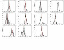
Analysis of the !selected! 360MeV (including 4.4MeV and 9.6 MeV excited states)
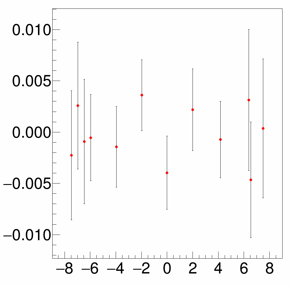
With the new discovery in mind, I removed the problematic points, ie, keeping only first seven (0, 2.5, 5, 7.5, -7.5, -5, -2.5).
With only these points (including their excited states) the results improved significantly.
However, improvements are still needed.
30.)  31.)
31.) 
32.)  33.)
33.) 
Last modified 11.1.2017


 05.)
05.) 

 09.)
09.) 
 11.)
11.) 

 14.)
14.) 
 16.)
16.) 
 19.)
19.) 
 21.)
21.) 

 25.)
25.) 
 27.)
27.) 


 31.)
31.) 
 33.)
33.)