Meeting No. 20
Normalization of the FFs
In our Skype meeting we discussed the problem with normalisations.
You could see how important this is for the extraction of our radius. I was afraid
that changing the normalisations of the FFs after already normalising the
cross-section ratios to 1 brings unwanted bias to our analysis. My main
concern was the following:
If the normalisation of the cross-sections would be chosen poorly, (for instance
0.5% away from 1) this offset is not compensated by the open normalisation of the FFs,
because both ISR and FSR parts are contributing to the CS. Hence, because of
mixed contributions to the CS we need to be careful how we transform the
extracted CS ratios to the FFs.
Our CS ratios are scattered around 1. These small deviations from one we then correlate
to the relative offsets of the FFs from a chosen model. In our case, Jan's model. In this procedure
we assume that the whole shift is a consequence of the ISR part, i.e., form-factor
at the given Q**2 point. This means, that we are intrinsically assuming, that
FF at the elastic peak is precisely known and that this point matches
exactly Jan's model. If this is so, then we should not change the normalisation
of the FFs again, because then we change also the Elastic FF, which was already
perfect.
Of course, without the elastic points it is a bit difficult to choose a proper normalisation.
Two normalisations were considered: 1.) Normalising the average of each data set to
one; 2.) Normalising the average of first two points to one. Since these two
points are close to the elastic, one then assumes that also the elastic points
is there. As you could see, these two normalisations give different values for
the radius, i.e., 0.85fm and 0.89fm, respectively.
In the last few days I investigated this matter in more detail. Please see the attached
Mathematica file and my hand written notes (that I will explain on the way).
MihaISRNotes181016.pdf
FitFormFactorsOctober.pdf
Now let's change the normalisation of the data for "dn", which shifts both parts of
the cross-section up, but we assume, that only ISR part is responsible for the change.
We get Eq.D. Now let's see, what happens, if we put this into our algorithm, that
we use to transform CS to FF. As mentioned before, we assume that the relative
difference in CS dR is contributed only by ISR. Then we use Eq. E to transform from
CS to FF. The factor a is obtained with the simulation.
Using Eq.D in Eq.E one sees that the relative difference in form-factor dGE is
proportional to dn. If a=const than the relative difference is constant and this means
than changing the normalisation really changes only the normalisation of the form-factor.
If so, that we can leave the normalisations of the FFs open and determine them
with the Minimisation algorithm. See Eq. G.
However, the parameter a is not constant but changes with Q2, because with Q2
the ISR/FSR ratio changes, as well the form-factors. For illustration see Eq. I.
Using some estimates, the parameter a changes from 1 at elastic line to 0.8 at
the end of the tail, mostly because ISR there contributes more than FSR to the cross-section.
Influence of the FF itself is not so large. Hence, for the first guess, we can parameterise
the change of the form-factor with a linear function as shown in Eq. K.
If we now put this into our model for the FF, we see that such function beside normalisation
now changes also the radius, according to Eq. N and Eq. O. From this we learn
that we need to be careful about choosing the right normalisation. However, from the
analysis in the Mathematica file you will be able to see, that this is not critical, because
of our limited precision on radius.
So. After this introduction, I redid the fitting of my data by leaving the three normalisations
open, as you suggested. This shifted my radius to even smaller value, i.e. 0.81fm. Then I
tried to see what happens to the result, if I normalise the CSs to the average instead of the
first two points. Furthermore, I also investigated, how the result changes, if I introduce small
positive and negative offsets to the cross-sections. I determined, that normalisations
of the fits compensate for this change. The radius also changes, but only little, i.e.,
for far less than what is our uncertainty.
In conclusion, With the open normalisations we get a robust result, which depends only
little on the chosen normalisation of the CS. I am sorry that I have not investigated this
earlier. Furthermore, the changes are comparable with what I guessestimated in my notes.
In the old approach, when I had two parameters for the whole data set I used a covariance
matrix to determine the error bars. With this "hybrid" fit I decided to determine the error of the
radius and normalisations by smearing the data with the gaussian distribution and checking
how do the radius and normalisations change. With the new way of fitting, the statistical uncertainty
increased from 0.02 to 0.035fm. Furthermore, when considering also the systematic uncertainty
the total uncertainty of the radius increased to 0.06fm. To my surprise is the reduced Chi**2 of the
fit with Sys. errors almost perfectly one. :)
Now I need to see, how the analysis behaves, if I consider this new radius in my analysis
instead of Jan's model. Unfortunately, this takes few days on my computer.
CF Model
I considered CF parameterisation as suggested by Marc. I adjusted the parameters
of the model such, that I get the same values for higher momenta. As I result I get a
slightly smaller radius, but consistent within our uncertainty.
Two photon
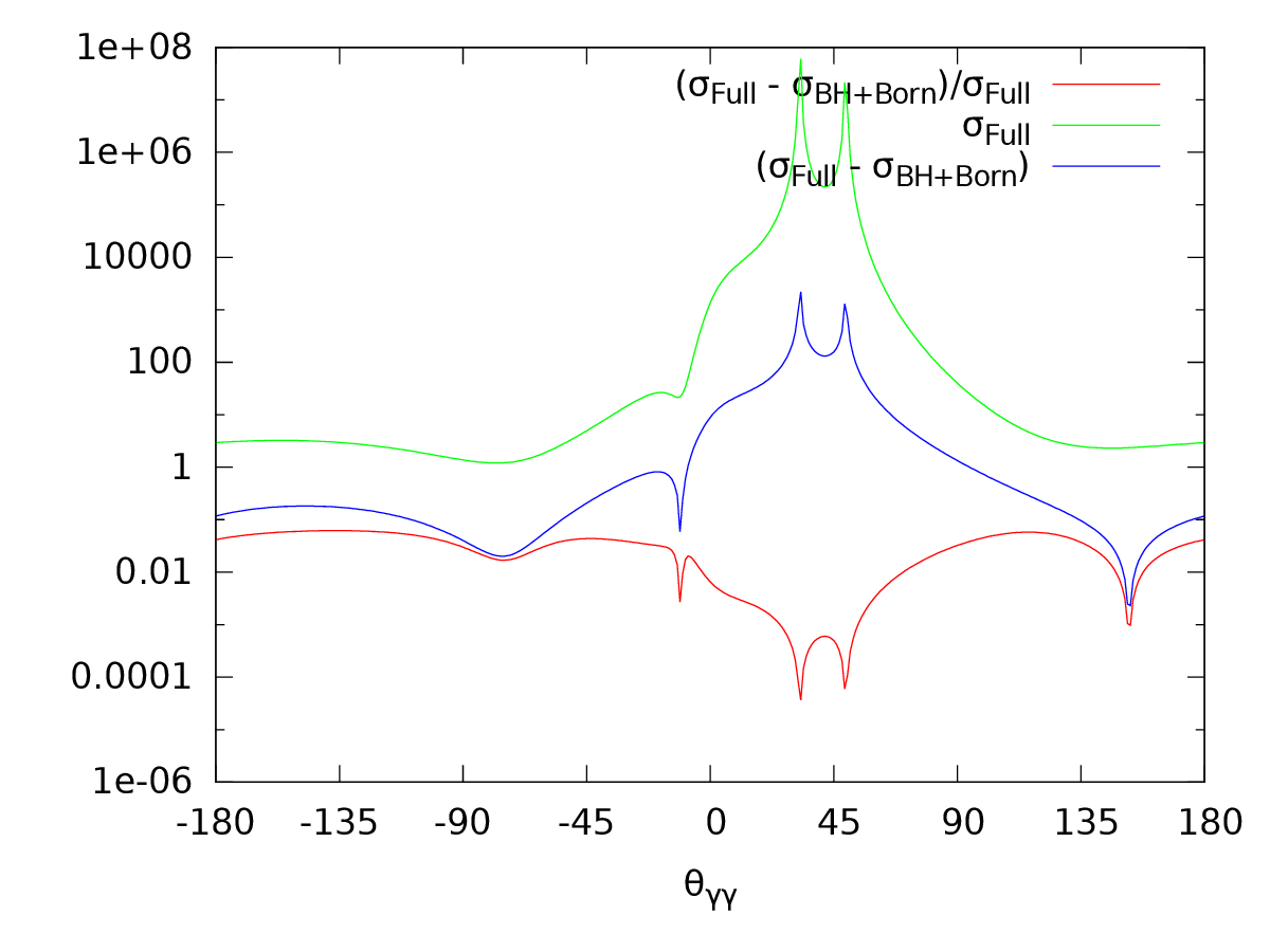
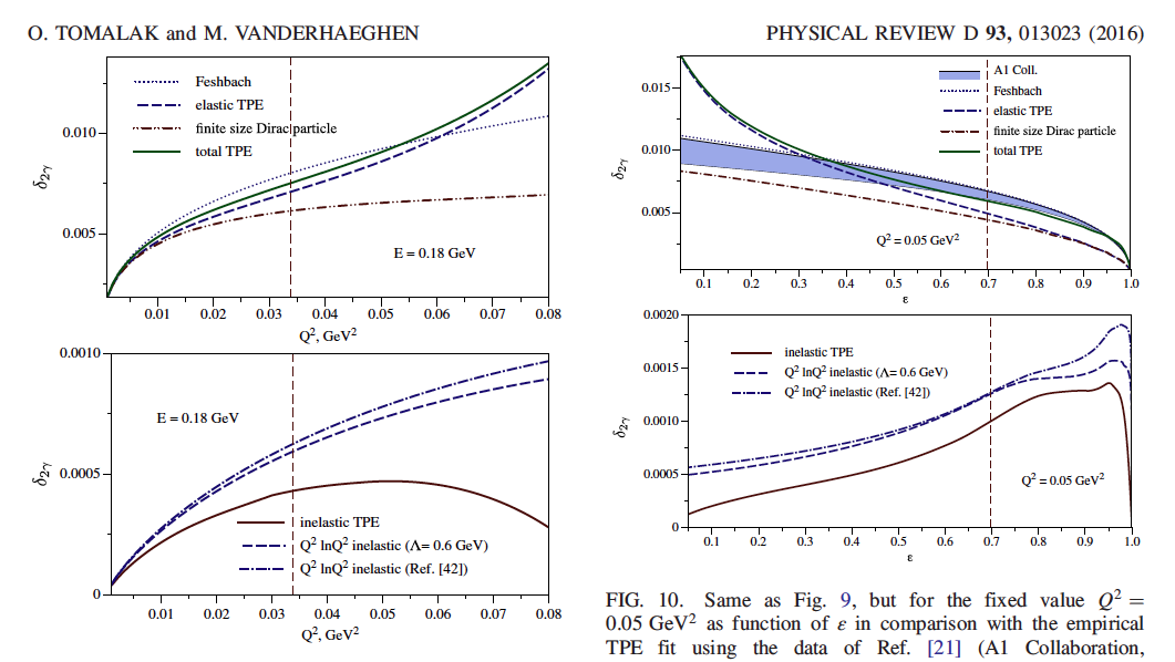
After receiving number from Adrian regarding the Two-photon
corrections I also investigated the effect myself. Using
Feshbach formula I got the same relative correction as Adrian, i.e.,
2.7E-3. This is a fixed number since correction depends only on the
angle. I went further and checked paper from Olexander and Marc,
which calculated TPE for similar kinematics. Please see Fig.
Tomalak.png. There you can see, that the full correction is indeed
at the level of 0.25%, for all the energies. Please keep in mind
that our epsilon = 0.96. Furthermore, we have on-shell correction
included in our calculation, which means that only off-shell part is
missing. According to Marc and Olexander, this contributions are
for our kinematics smaller than 1E-4, regardless of the kinematics
(of course, always assuming elastic limit).
1.) 
VCS using ChPT calcualtion in Cola++
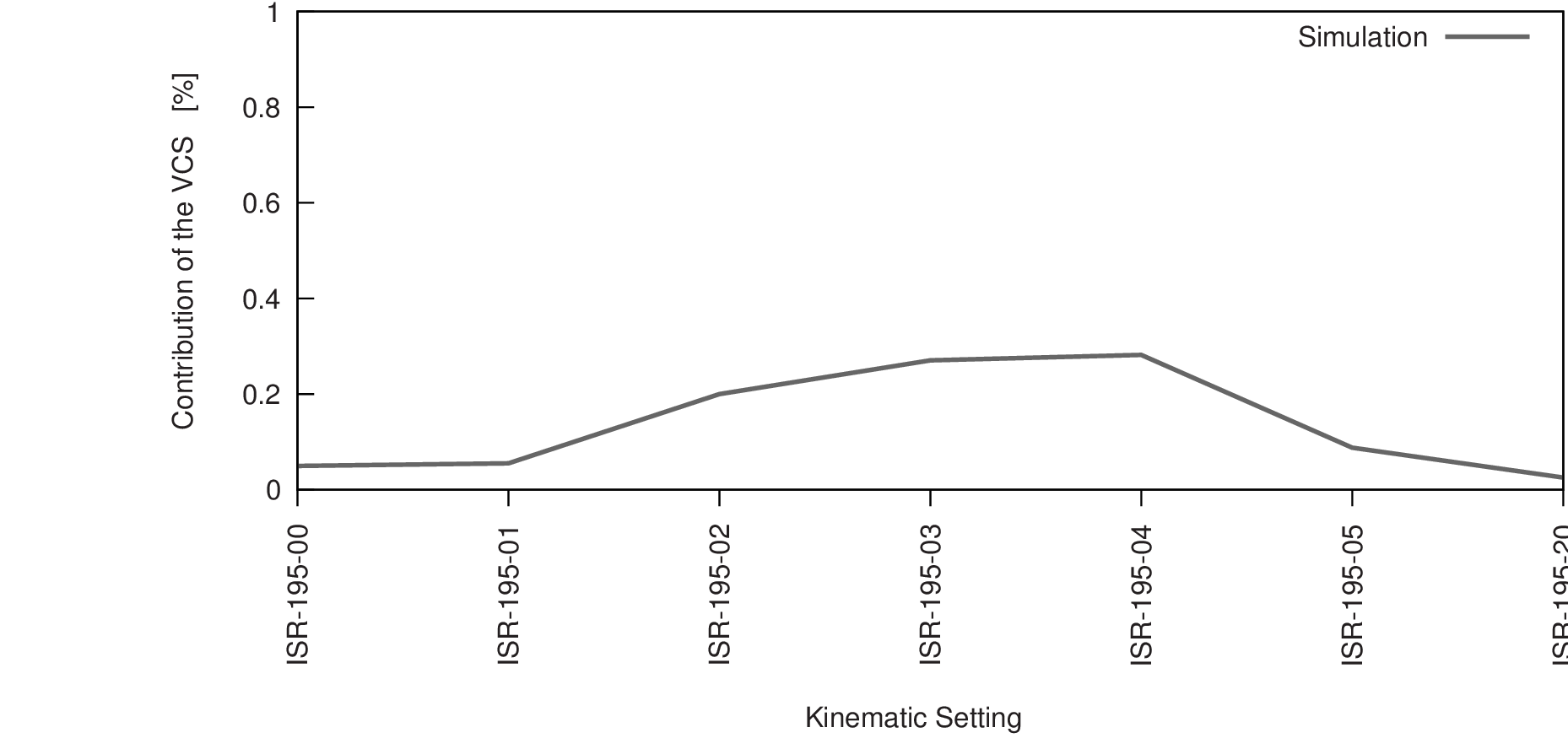
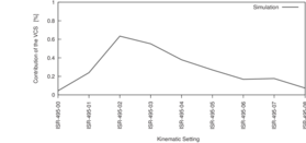
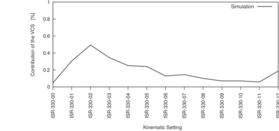
I tried to estimate the contribution of the VCS diagrams to our
simulation. For this I first I got a code from Jure, which I can not
compile. Instead, I considered code from Luca Doria, which is already
included in Simull++. I considered VCS model and ran the simulation
once with and once without BH-part (i.e., only off-shell Born part). This
gave me the estimate for the VCS contribution to our simulation.
The plots VCSContributionRatioPlots*.pdf show the results that I got,
and you can see, that contributions can be (to my surprise) <= 0.6%.
The most affected are the first two points in each kinematic.
2.)  3.)
3.)  4.)
4.) 
VCS correction by Harald
Harald brought back to life Marc's calculator, that uses isobar model.
He calculated the correction for Ein=330MeV, Eout = 230MeV, thetaE=15.2deg
and obtained much smaller correction. This is to his opinion also much more
realistic. Quick averaging over our acceptance gives a correction in order
of 10E-4, which can ne neglected in our calculation. Hence, we keep the
0.82fm result.
5.) 
Systematic undertainty:
I considered Jan's advice and divided systematic uncertainties on point-like and
slope-like parts. The point-like uncertainties change each point in different
direction. The slope-like uncertainties change all the points in the same direction
but for different values.
Results:
6.) 
7.) 
8.) 
Last modified 28.10.2016
 3.)
3.)  4.)
4.)