Meeting No. 17
The Analysis of the Target Frame contribution from January
One of the background contributions is the contribution from the target frame.
I estimated this contribution at the beginning of the year using approach described here.
The following three plots show the contribution of the target frame to the measured spectra for the
three beam energies.
01.)  02.)
02.)  03.)
03.) 
To get rid of the Tg. frame correction in the analysis we consider a theta0 cut [-3.8, -1], which
represents the upper part of the acceptance. The following plot shows the difference in the vertex
spectrum using difference in the vertex spectra using different theta0 cuts. The upper plot shows
the full spectrum (cyan) together with the spectrum with nominal theta0 cut considered in the
analysis (purple). The bottom two plots show (properly rescaled to the same number of bins)
the difference between nominal (purple) distribution and distribution with cut [-3.8, -3.5].
04.) 
Now it is interesting to see, how the results change if
different interval is considered. The easiest thing is to compare the integral of the vertex plots
for different theta0 ranges, ie. R(x) = Vertex(-3.8,x)/Vertex(-3.8,1), for different cuts on Vertex-Z.
One sees, that when moving along the theta0 the ratio is not flat, as I had expected. It seems, that
acceptance is still large enough that CS depends on the out-of-plane angle. To get rid of the effect
we need to apply more strict cuts on Vertex-z. More strict was the cut, more consistent are the
results.
05.) 
Hence, I decided to use in the analysis vertex cut [0,10]mm. To estimate the residual effect
of the Target frame, I compared the ratio with the one with the cut [5,10]mm (rescaled to the
same number of bins). This is show on the plot below:
06.) 
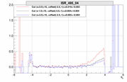
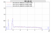
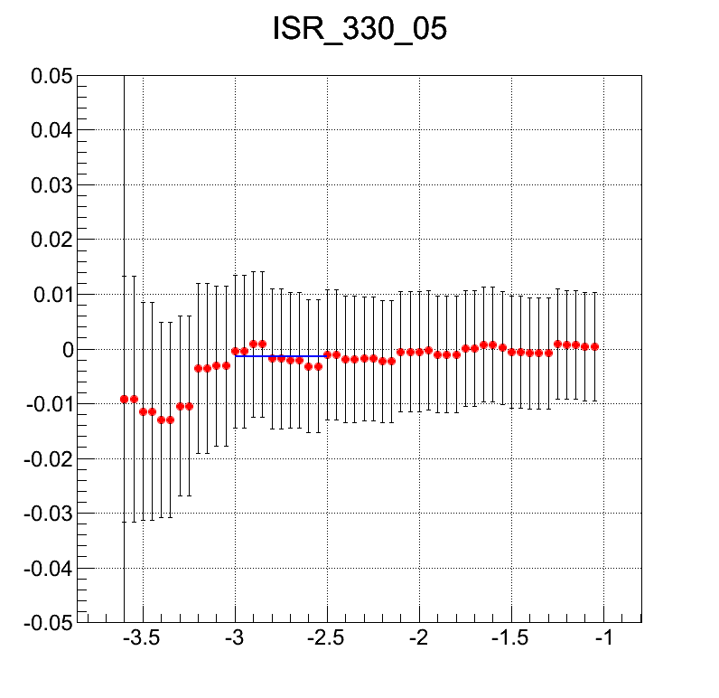
Then I fitted this ratio in the region between [-3.0, -2.5] in order to get correction parameter
and the corresponding error. This region was chosen because in assume that the region from the minimal
angle up to -2.5 is clean of background and I need to compare this to the values I considered in my
analysis. Furthermore, I did not go completely to the minimum of -3.8 but only to -3, where the
region is not affected by the effects on the edge.
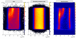
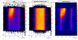
Rethinking this correction
After rerunning the analysis and getting final results I got disturbed by the jump in the correction
at kinematics 495-03. This is not "physical. I revisited the correction and was not happy with it any more.
The reason why I did the correction this was is because I did not want to compare with the simulation.
I was afraid that if I compare with simulation, I will endanger final result. However, this can be avoided.
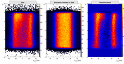
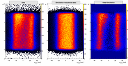
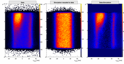
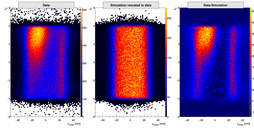
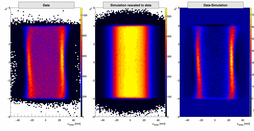
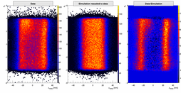
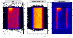
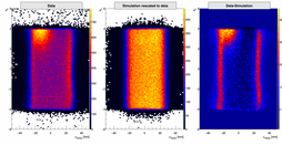
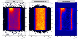
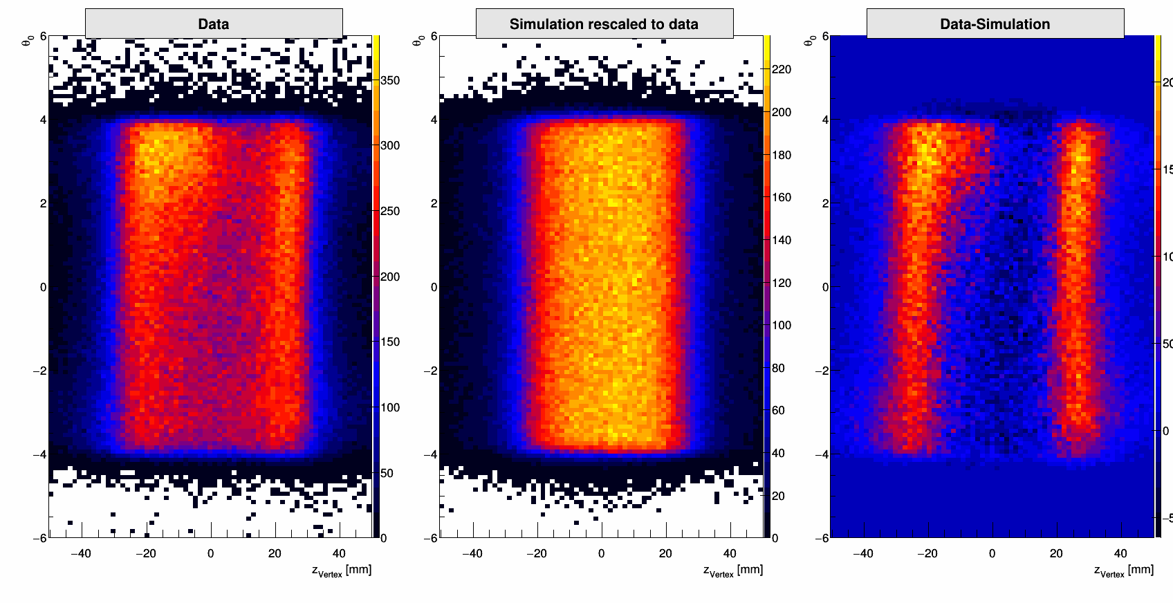
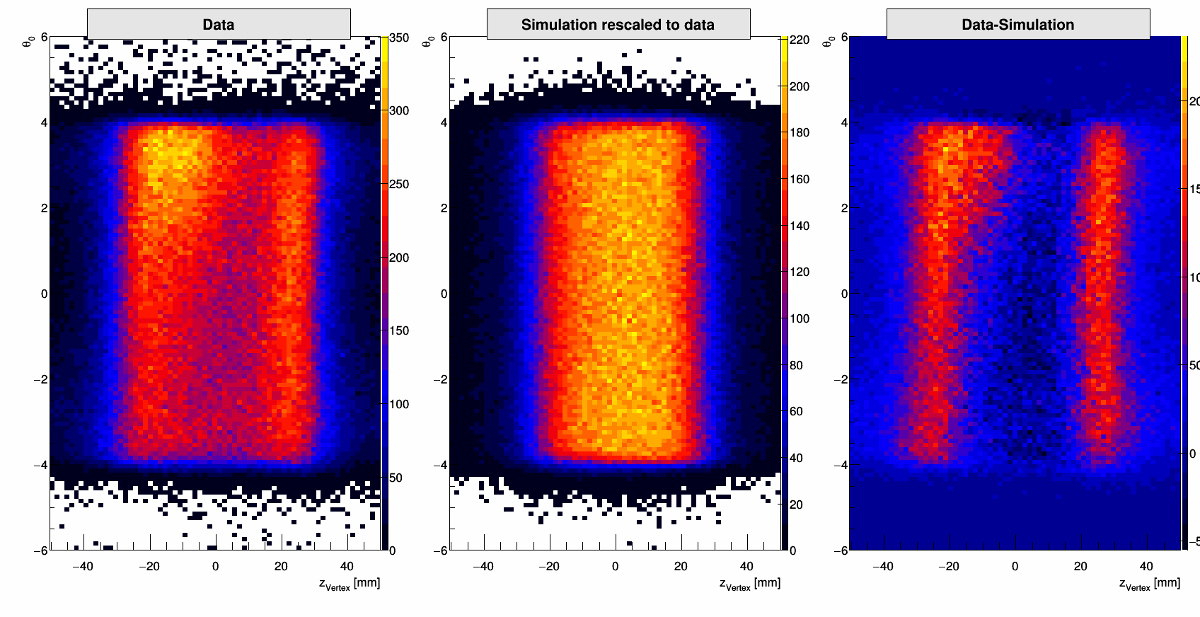
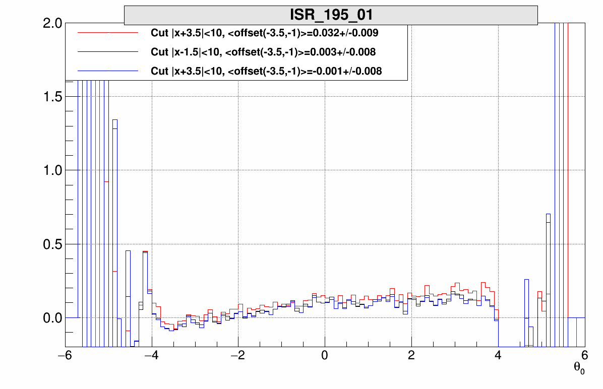
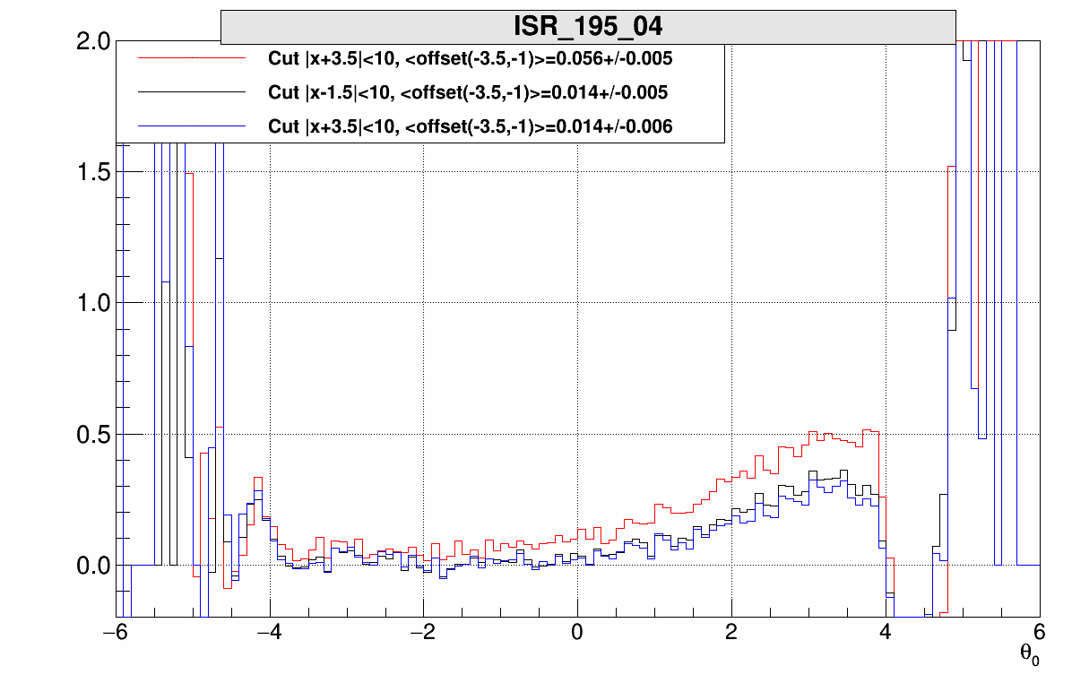
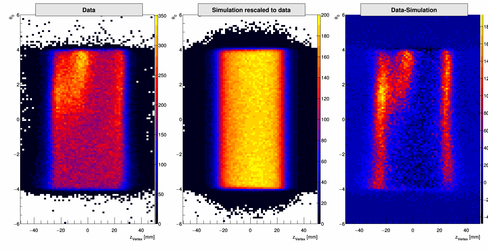
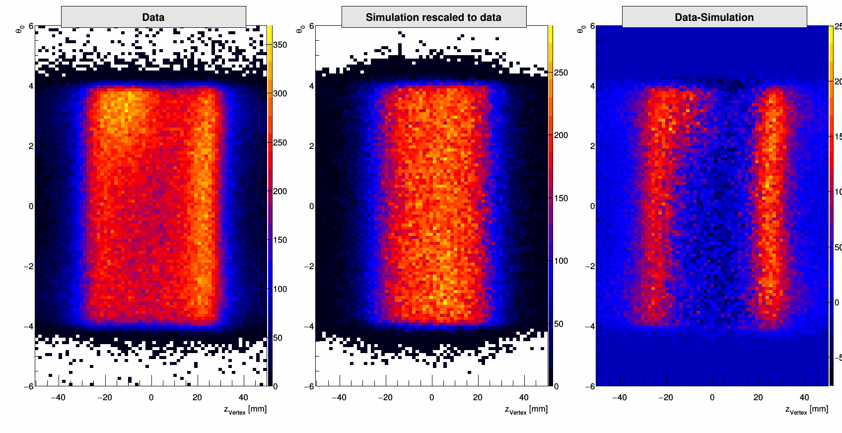
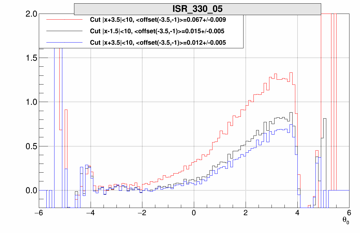
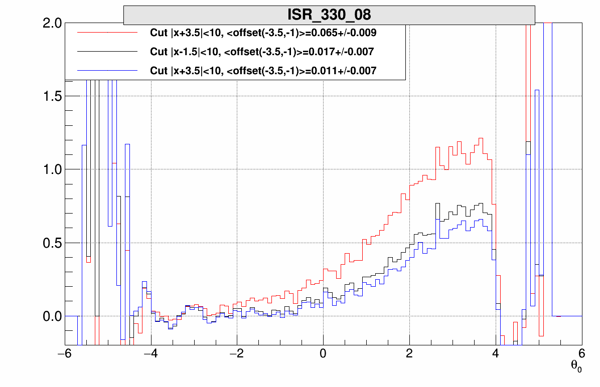
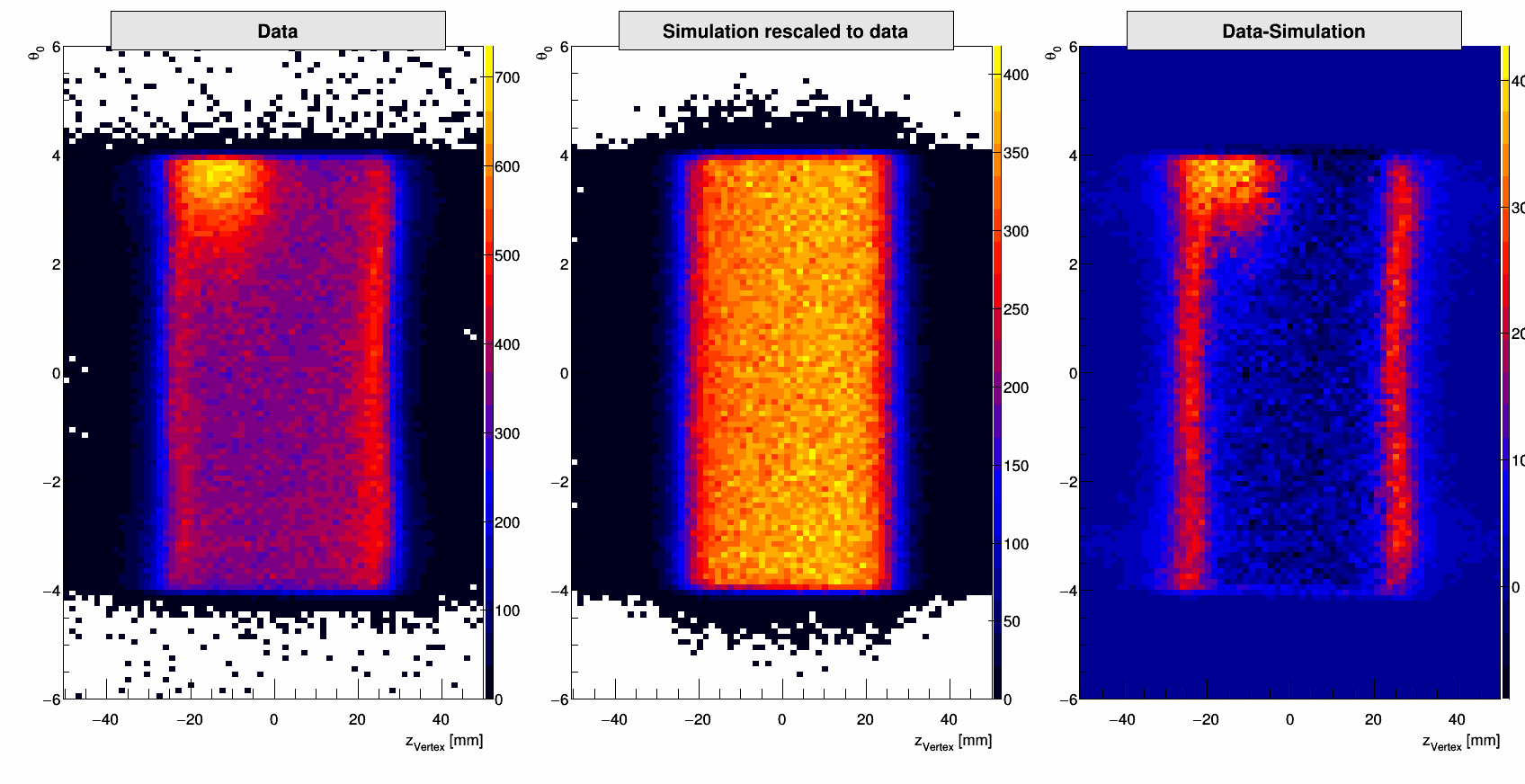
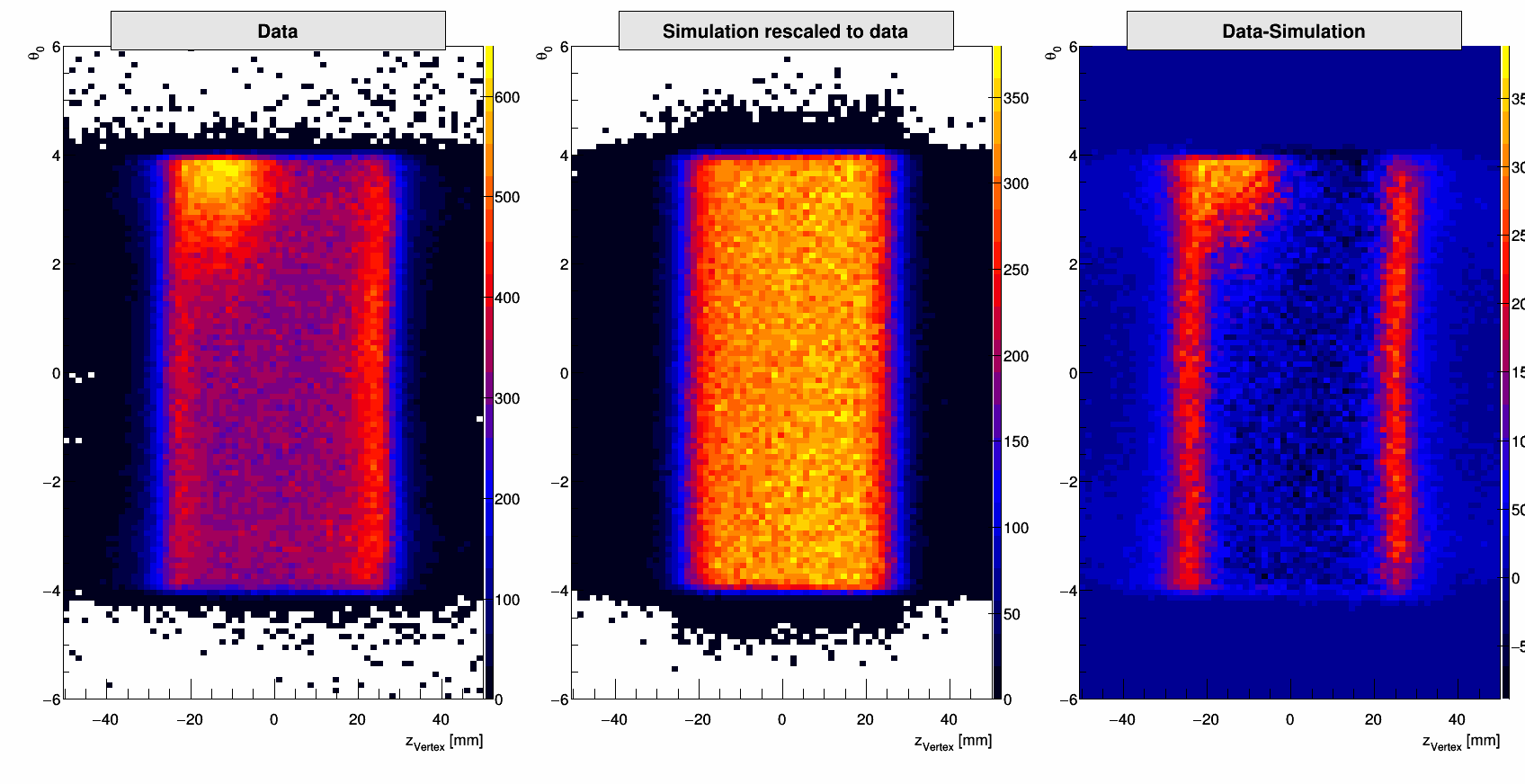
Therefore, I did the following approach: First I plotted the data. I selected a clean region in the vertex vs. theta0 plot.
Then I plotted the simulation. Assuming that the whole acceptance has only 1 cross-sections and that the whole
functional dependences (ie. all slopes that we see) are due to the acceptance, I renormalized the simulation
to the data, using the number of events in the clean region. This way I got rid of the problem with the FF.
Then I compared the data and simulation, ie, calculated the difference to observe the extra contribution of the
frame. Then I selected thee regions along the vertex-z axis. Each band has the same length as the cut in the
analysis. I selected one to the left of zero, where the problem is, one around zero and I above zero, where
the problem is "minimal". Then I compared, how much the region considered in the analysis differs from the
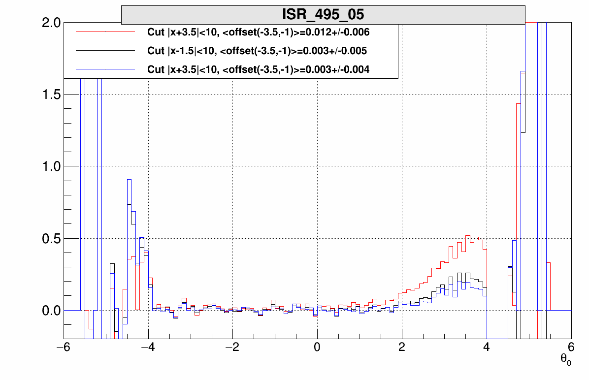
"contaminated" and "clean" region. One can see, that in the selected theta0 range [-3.8, -1], one can
not see a significant difference between the clean (blue) and chosen region (black). However, for some
kinematics, where the contamination is the largest, one can see the difference between selected (black)
and contaminated region (red). Hence, I concluded, that the contribution I added is overestimated and
should be removed from the results. Here are the results:
ISR-195:
07.)  08.)
08.)  09.)
09.)  10.)
10.) 
11.)  12.)
12.)  13.)
13.) 
14.)  15.)
15.)  16.)
16.)  17.)
17.) 
18.)  19.)
19.)  20.)
20.) 
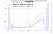
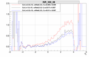
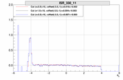
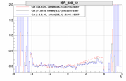
ISR-330:
21.)  22.)
22.)  23.)
23.)  24.)
24.) 
25.)  26.)
26.)  27.)
27.)  28.)
28.) 
29.)  30.)
30.)  31.)
31.)  32.)
32.) 
33.) 
34.)  35.)
35.)  36.)
36.)  37.)
37.) 
38.)  39.)
39.)  40.)
40.)  41.)
41.) 
42.)  43.)
43.)  44.)
44.)  45.)
45.) 
46.) 
ISR-495:
47.)  48.)
48.)  49.)
49.)  50.)
50.) 
51.)  52.)
52.)  53.)
53.)  54.)
54.) 
55.) 
56.)  57.)
57.)  58.)
58.)  59.)
59.) 
60.)  61.)
61.)  62.)
62.)  63.)
63.) 
64.) 
Removing this correction from the analysis changes the final result and requires rethinking of the
corrections. Comes next. Additionally, I revisited also other corrections and they all seem
robust and consistent!!!
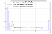
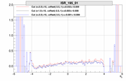
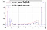
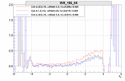
MAID Uncertainty
I meet prof. Tiator and asked him about the MAID uncertainty at the threshold, which
is important for our results and effects our final systematical uncertainty. He said,
that the best way to see this would be to compare different MAID models. And this is
what I did. Below see the results of the comparison. The two red lines on the bottom
plot show the weighted uncertainty of the MAID 2000 used in Cola with respect to the
MAID 2007 for Pi+. One can see, that the 5% uncertainty has been a good guess for the
uncertainty. Hence, considering that the MAID brings 10% of the events, is the final
uncertainty 0.5%.
65.) 

 03.)
03.) 


 08.)
08.)  09.)
09.)  10.)
10.) 
 12.)
12.)  13.)
13.) 
 15.)
15.)  16.)
16.)  17.)
17.) 
 19.)
19.)  20.)
20.) 
 22.)
22.)  23.)
23.)  24.)
24.) 
 26.)
26.)  27.)
27.)  28.)
28.) 
 30.)
30.)  31.)
31.)  32.)
32.) 

 35.)
35.)  36.)
36.)  37.)
37.) 
 39.)
39.)  40.)
40.)  41.)
41.) 
 43.)
43.)  44.)
44.)  45.)
45.) 

 48.)
48.)  49.)
49.)  50.)
50.) 
 52.)
52.)  53.)
53.)  54.)
54.) 

 57.)
57.)  58.)
58.)  59.)
59.) 
 61.)
61.)  62.)
62.)  63.)
63.) 

