Meeting No. 1
Converting measured CS offsets to FF:
To be able to calculate FFs from the measured CS differences in the tail
region, we need a transformation function, which tells us, how differences
in CS reflect differences in the FF. The corresponding function for all
three energies is shown below:
01.) 
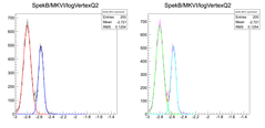
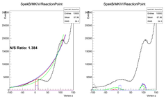
To get this function I considered our simulation. For each kin. setting I
ran simulation 5 times, each with different scaling of the form-factor
(-2%,-1%, 0%, +1% +2%). However, when scaled, both ISR and FSR get scaled.
Hence, to get the effect of the ISR only, I need to compare ISR(scaled) + FSR(unscaled)
with the ISR(unscaled)+FSR(unscaled). This can be done, by looking at the
simulated Vertex-Q2 histograms, fitting the peaks to identify the ISR and
FSR parts and then do the comparison. The plot below shows the
spectrum for 0% simulation on the left and 2% percent simulation on the
right.
02.) 
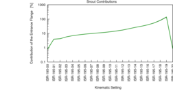
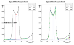
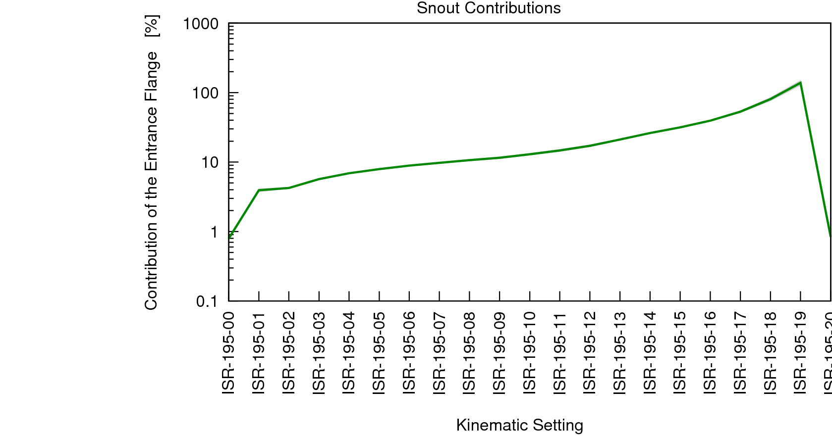
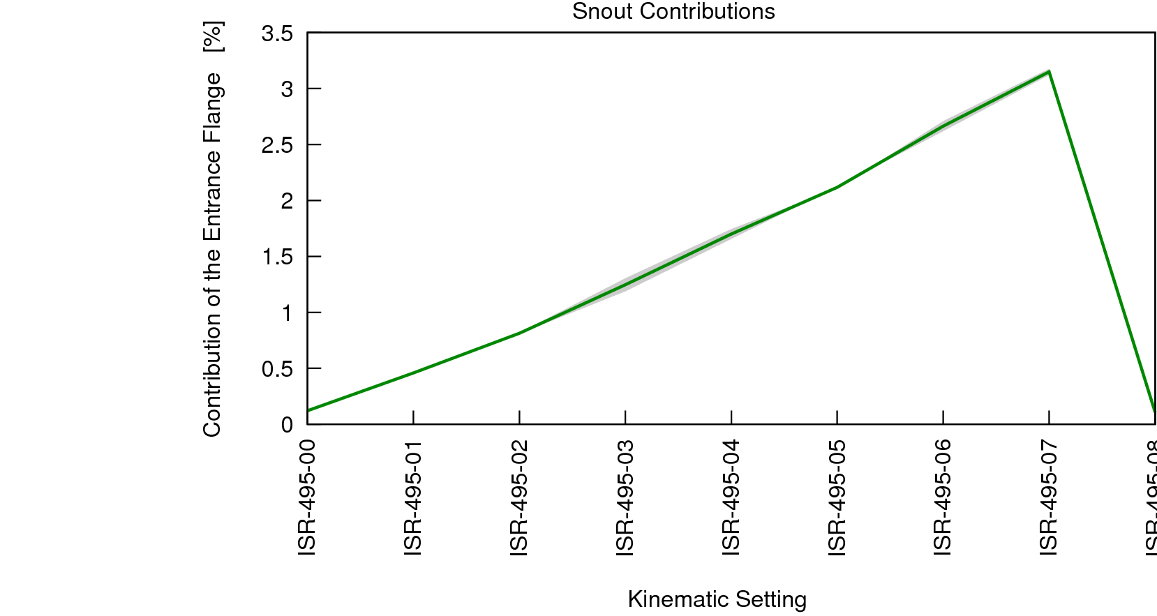
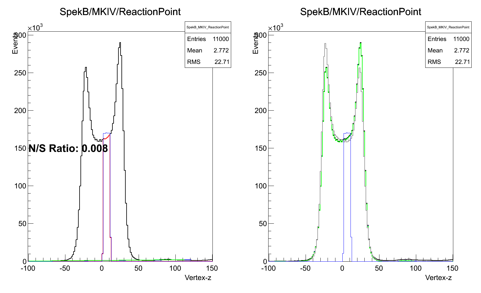
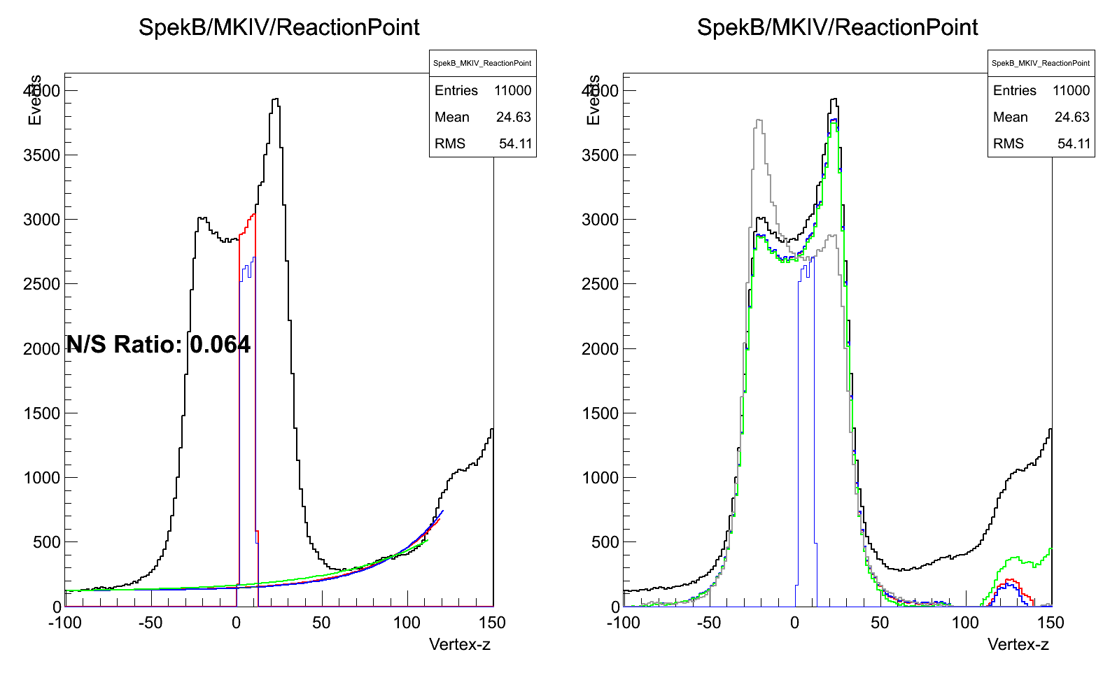
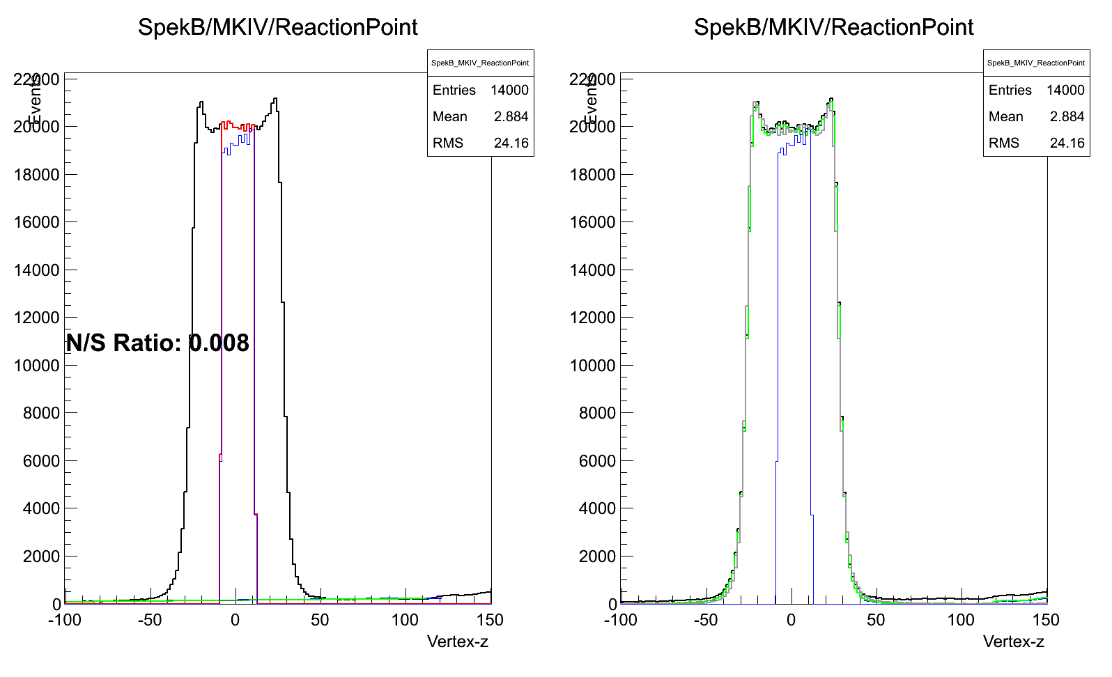
Analysis of Snout contribution
Following three plots show the size of the snout effect. This contribution needs to
be subtracted from the measured CS ratios, in order to get proper results. The corrections
are small for the 495MeV setting but very large for the 195MeV setting.
03.)  04.)
04.)  05.)
05.) 
The size of the correction was determined by estimating how much snout contributes to
the measured spectra, by looking at the Vertex plot after performing all the other
cuts. The background was parameterized with the exponential function, using data
to the left and to the right of the target. The uncertainties were estimated by
comparing exponential functions with different ranges. Once determined the fit, I subtracted
the background from the data. I was happy with the fit, when the "clean spectrum"
matched with the flipped spectrum, assuming left/right rotational asymmetry for
the clean spectrum. The following plots show the details of the analysis for
the three energy settings:
195MeV (0, 5, 10, 19)
06.)  07.)
07.)  08.)
08.)  09.)
09.) 
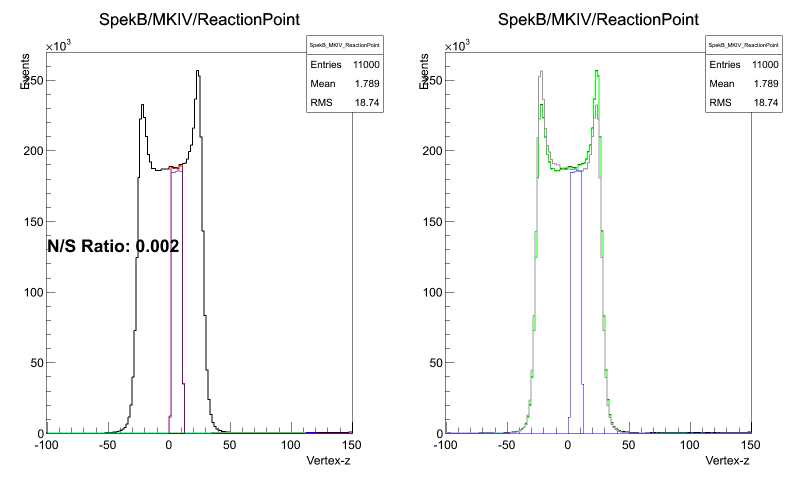
330MeV (0, 3, 5, 10)
10.)  11.)
11.)  12.)
12.)  13.)
13.) 
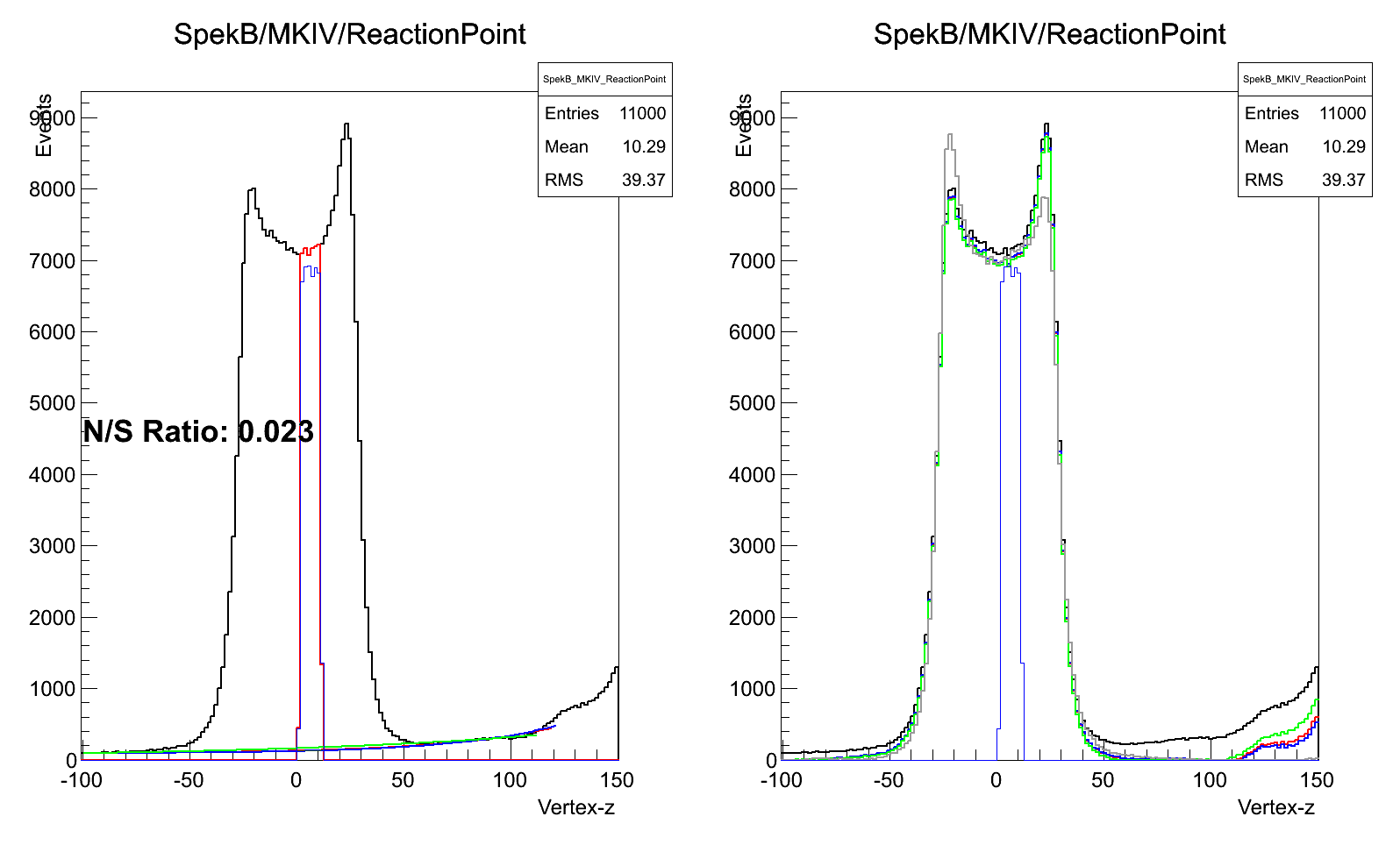
495MeV (0, 2, 4, 7)
14.)  15.)
15.)  16.)
16.)  17.)
17.) 
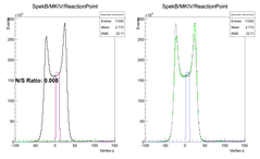
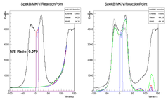
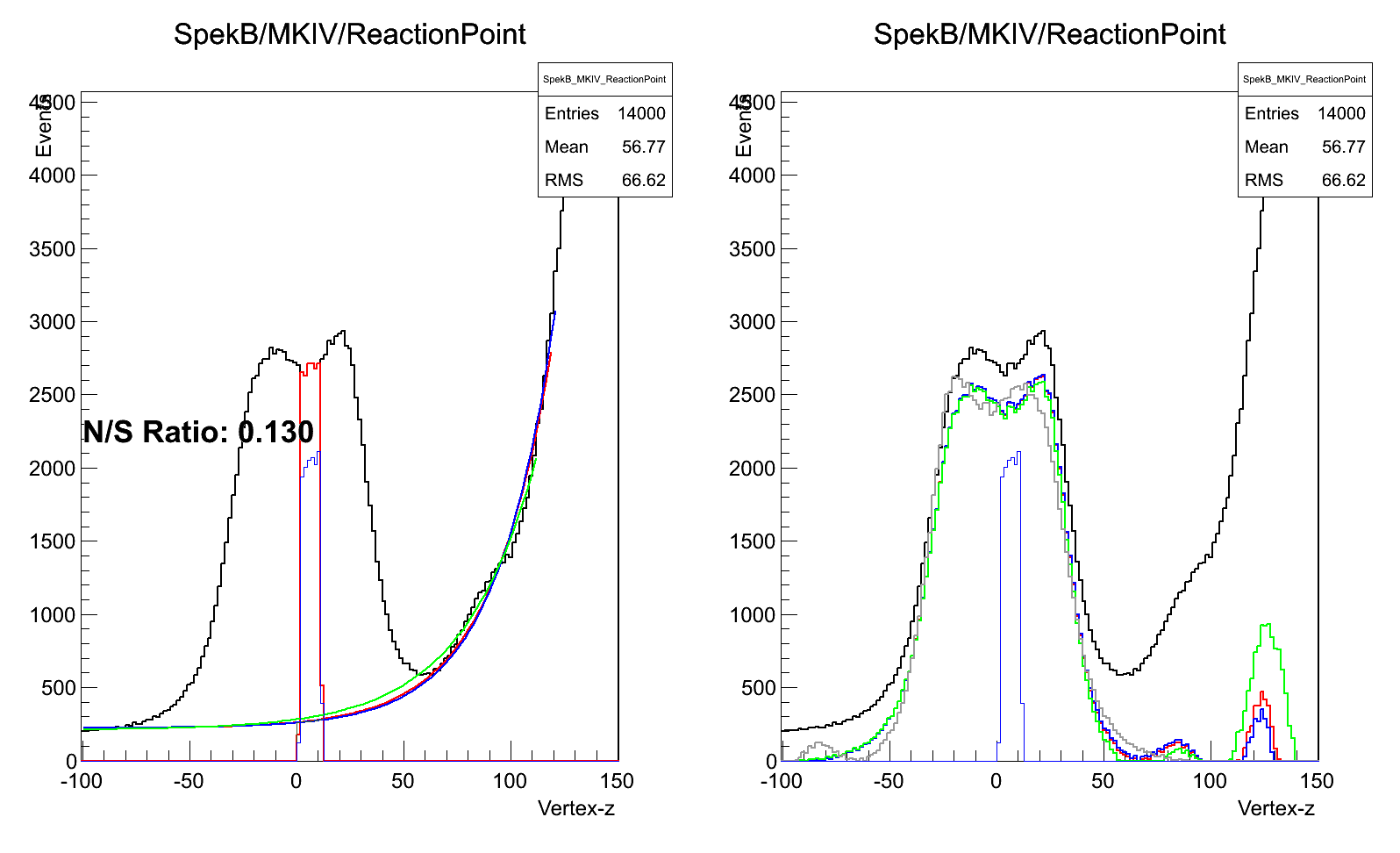
Analysis of the Target Frame contribution
The following three plots show the contribution of the target frame to the measured spectra for the
three beam energies.
18.) 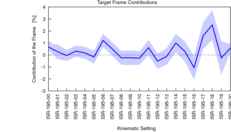 19.)
19.) 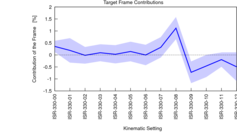 20.)
20.) 
To get rid of the Tg. frame correction in the analysis we consider a theta0 cut [-3.8, -1], which
represents the upper part of the acceptance. Now it is interesting to see, how the results change if
different interval is considered. The easiest thing is to compare the intergral of the vertex plots
for different theta0 ranges, ie. R(x) = Vertex(-3.8,x)/Vertex(-3.8,1), for different cuts on Vertex-Z.
One sees, that when moving along the theta0 the ratio is not flat, as I had expected. It seems, that
acceptance is still large enough that CS depends on the out-of-plane angle. To get rid of the effect
we need to apply more strict cuts on Vertex-z. More strict was the cut, more consistent are the
results.
21.) 
Hence, I decided to use in the analysis vertex cut [0,10]mm. To estimate the residual effect
of the Target frame, I compared the ratio with the one with the cut [5,10]mm (rescaled to the
same number of bins). This is show on the plot below:
22.) 
Then I fitted this ratio in the region between [-3.0, -2.5] in order to get correction parameter
and the corresponding error. I just need to reconsider why I have chosen this range?!
Latest results:
Following two plots show the present status of the results. I have added the 195MeV data so that
we can now see the full range in Q2 that we can cover. Furthermore, I have now properly considered
the Snout and Frame contributions for the 495MeV setting. In the previous analyses, this was done
by a simple approximation. Now I as still trying to determine the best RadCorrFac factors for the
elastic settings. Once I will know them, I will run the simulation with full statistics.
23.) 
24.) 
Simulation with the Lupolen target:
I have started working on a simulation to see, if the solidstate (Lupolen) target can be used
for the ISR experiment. The idea is measure each setting with Lupolen and Carbon targets, and
then subtract the two to isolate the Hydrogen spectrum. The question is, how well can we do this.
Therefore, I added a new model to the Simul++, which simulates Lupolen target (in the first order
Peaking approximation). I compared my results with the data taken during the Calib2014 beam time.
Unfortunately are the data available only for spectrometer A. Although the C12 peak dominates,
the H spectrum is still clearly visible. Furthermore, when running at low Q2, the excited states
will disappear and there will also be no QE peak at low E'.
25.) 
In the next step I will improve this first attempt and consider our full Hydrogen simulation
in order to get a feeling how much statistics would be needed for such experiment and
what is the precision that we can expect.


 04.)
04.)  05.)
05.) 
 07.)
07.)  08.)
08.)  09.)
09.) 
 11.)
11.)  12.)
12.)  13.)
13.) 
 15.)
15.)  16.)
16.)  17.)
17.) 
 19.)
19.)  20.)
20.) 


